To be honest, RankMyPhoto is a pretty skeezy website. It encourages objectification and seems like a big cry for attention. The premise is you upload a photo of yourself and anonymous internet users can rank your attractiveness and also vote you “Hot” or “Not”. But they do have good data.
I built a python script to scrape about 9000 profiles for their biographical data. Unfortunately, height, weight, eye color, and hair color are all text inputs so there was far too much variation to do any analysis on them. But other factors such as age, education, alcohol/tobacco use, body type, etc. are consistent across profiles. I wanted to do two things with this data: first explore it to see if there are any interesting correlations and second, see if the data are significant to predict attractiveness.
Although they are not perfect, generalized linear models continue to be one of the most commonly used tools in statistics. R makes building these models very easy and my first step was to split out the data into training and test sets. I also had to remove some bad data.
rmpdef<-read.table("pdatatab.txt",header=T,sep="\t",allowEscapes=F,quote="",comment.char="")
rmp<-subset(rmpdef,rmpdef$Age<=60
            &rmpdef$Rating>0
            &rmpdef$MaritalStatus!="Widowed")
rmp<-rmp[rmp$Alcohol!="Often",]
filter<-as.logical(rbinom(nrow(rmp),1,.8))
rmptrain<-rmp[filter,]
rmptest<-rmp[!filter,]
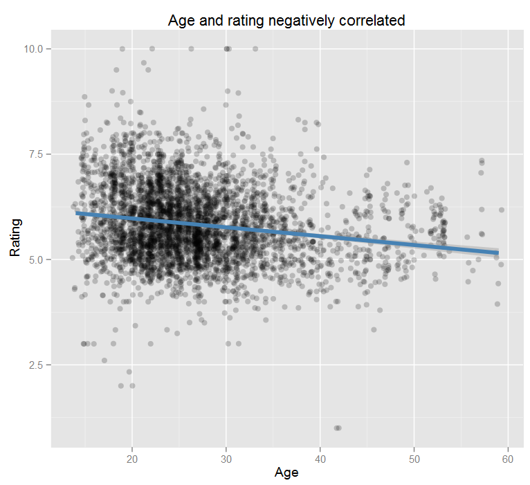
My first thought was to look at age and as expected, there is a strong correlation (p≈0).
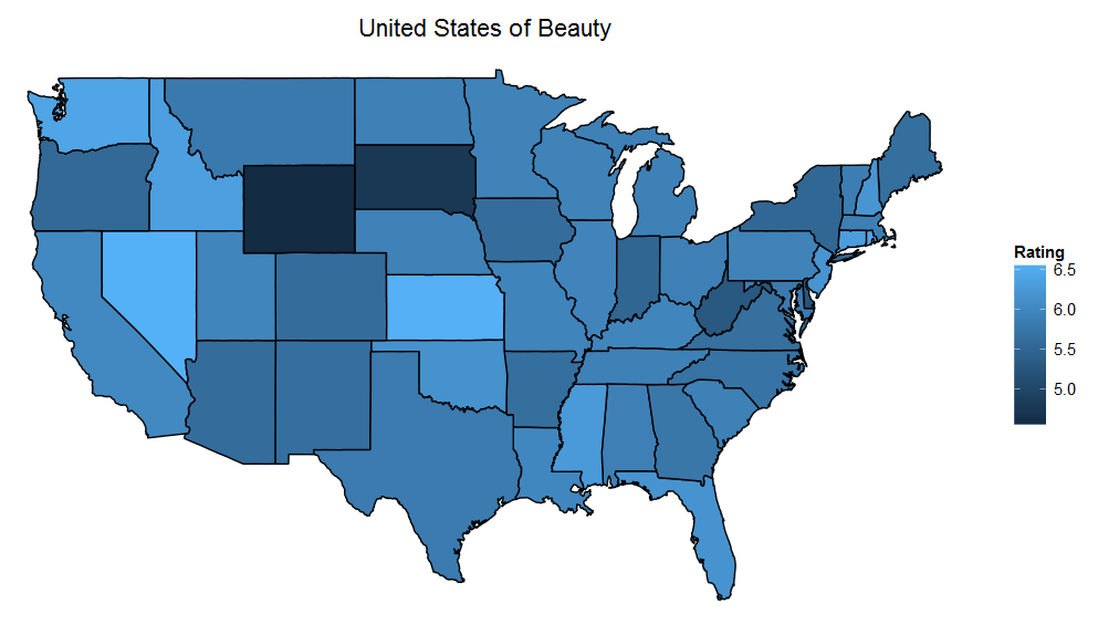
But as is usually the case with real-world data, you can get a better correlation when looking at more variables. I built a few models and tested them using cross validation, looking for the one with the highest accuracy. My most successful model included age, alcohol usage, body type, religion, state, sexuality, marital status, and education and it predicted attractiveness within ±10% on the test data.
> lm_best<-lm(Rating ~ Age+Alcohol+BodyType+Religion+State+Sexuality+MaritalStatus+Education,data=rmptrain,na.action=na.omit)
> pred<-predict(lm_best,newdata=rmptest,na.action=na.pass)
> summary(abs((pred-rmptest$Rating)/rmptest$Rating),na.rm=T)
   Min. 1st Qu.  Median    Mean 3rd Qu.    Max.    NA's
 0.0001  0.0370  0.0876  0.1181  0.1592  2.1420     844
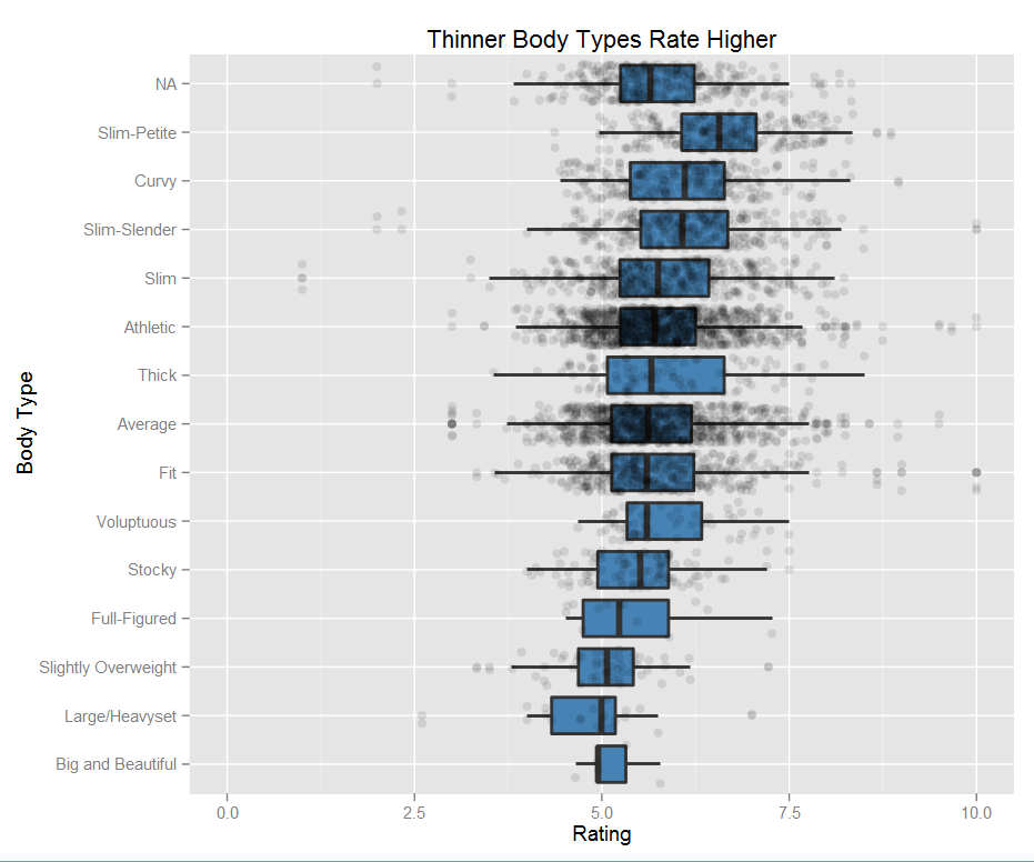
While I think it’s interesting that all of these data pieces correlate to rating, the one that I found most interesting was body type. Keeping in mind this data is all self-reported, the most common types were “average” and “athletic.” This graph shows the correlation between body type and rating with each point representing a person.
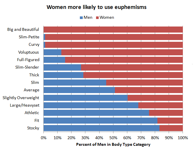
Some these body types are feminine in nature, so I also took a look at which types are more commonly used by men. I’m assuming that the voluptuous men are joking, but it is interesting to note that women prefer to use euphemisms for larger body types, whereas men use more direct terms.
I built a quick app that lets you play around with all of the factors I gathered. It uses the values that I got from my model in R to predict the attractiveness. Note that all fields are required for the prediction to be accurate.
And just for fun: