Method Chaining Gone Wrong

Method chaining is the feature available in many programming languages to stack method calls in one line, with each method accessing the object the previous method returned. Compare:

//Without chaining
MyObject obj = new MyObject();
obj.setVariableA("a");
obj.setVariableB("b");
obj.setVariableThree(3);

//With chaining
MyObject obj = new MyObject()
    .setVariableA("a")
    .setVariableB("b")
    .setVariableThree(3);

The first block’s MyObject class uses traditional setters whereas the second block uses setters that actually return the object being acted upon. This is often used in the Builder Pattern that creates objects with many optional parameters. Here is a brief example:

class Automobile{
	enum Color {
		RED, BLUE, BLACK;
	}
	
	private String make;
	private String model;
	private Color color;
	private double MSRP;
	private int horsepower;
	private int doors;
	private int weight;
	private int cylinders;
	
	public Automobile setMake(String make){
		this.make = make;
		return this;
	}
	
	public Automobile setModel(String model){
		this.model = model;
		return this;
	}
	
	public Automobile setColor(Color color){
		this.color = color;
		return this;
	}
	
	public Automobile setMSRP(double MSRP){
		this.MSRP = MSRP;
		return this;
	}
	
       //Remaining methods omitted for brevity

}

public class CreateCar{
	public static void main(String[] args){
		Automobile myCar = new Automobile()
			.setMake("Alfa Romeo")
			.setModel("8C")
			.setColor(Automobile.Color.BLACK)
			.setHorsepower(444)
			.setMSRP(250000.00d);
	}
}

(Note: There are improvements that should be made to this to truely fit the pattern. See this article for more details.)

However, there is no requirement that method chaining be used with the same object type. Consider something like Integer abc = myArrayList.get(0).get("abc");. Presumably, this code retrieves the map at position 0 in myArrayList and retrieves the Integer mapped to the String “abc.”

This is very tidy and can help to keep code clean, but unfortunately can introduce some problems. First, just looking at the code doesn’t tell me what objects are being called. My IDE will help me out by hovering over each section, but that can be annoying. Second, if something goes wrong on this line like a NullPointerExpection I need to go digging or use the IDE debugger to figure out what is null.

Unfortunately, here’s what happens when a developer goes off the rails:

systemImportDataBean.setType(converterMappingValues.getLocationMap().get(new StringBuffer().append(converterMappingValues.getDescriptionMap().get(systemImportDataBean.getPrimaryId().toLowerCase()).toLowerCase().trim()).append(FieldConstants.OTHER_LOOKUP.toLowerCase()).toString().toLowerCase().trim()));

NO, GOD! NO GOD, PLEASE NO. NO. NO. NO. NOOOOOOO!

Throw us a bone here and at least give us some line breaks! For…clarity(if that’s even possible):

systemImportDataBean.setType(
	converterMappingValues
	.getLocationMap()
	.get(
		new StringBuffer()
		.append(
			converterMappingValues
			.getDescriptionMap()
			.get(
				systemImportDataBean
				.getPrimaryId()
				.toLowerCase()
				)
				.toLowerCase()
				.trim()
			)
			.append(
				FieldConstants.OTHER_LOOKUP
				.toLowerCase()
			)
			.toString()
			.toLowerCase()
			.trim()
		)
	);

GL;HF when something goes wrong with this code. Please be kind to your fellow developers and don’t do something like this. Just because the compiler will let you do this doesn’t mean you should. The compiler isn’t the one will have to dig through this line to fix an error.

N-Queens Part 3: Success

In the last two posts we explored three different algorithms for solving the n-queens problem. If we wanted to actually implement one of them, we would need to consider which one performs the best. However, performance can be measured in a number of ways.

The first measurement of performance is simple–how effective is the algorithm at solving the puzzles? Remember that some of the algorithms can get “stuck” and therefore may not reach a heuristic cost of zero. Second we can look at the number of iterations the algorithm takes to solve the puzzle. Finally, the speed of the algorithm should be considered. An ideal algorithm is one that solves the most number of puzzles in the least number of steps and in the least amount of time.

In terms of success, both steepest hill climbing and annealing perform equally well (>90%), but first choice hill climbing falls short at only solving approximately 14% of problems. These also hold true regardless of the number of queens.

The annealing algorithm takes the most number of steps. This is because as the temperature drops, the algorithm is less likely to accept a move. Therefore, the algorithm takes several steps that do not result in making a move. The steepest hill climbing algorithm takes the fewest number of steps, solving 8 queens in 24 moves and 25 queens in only 35 moves, on average.

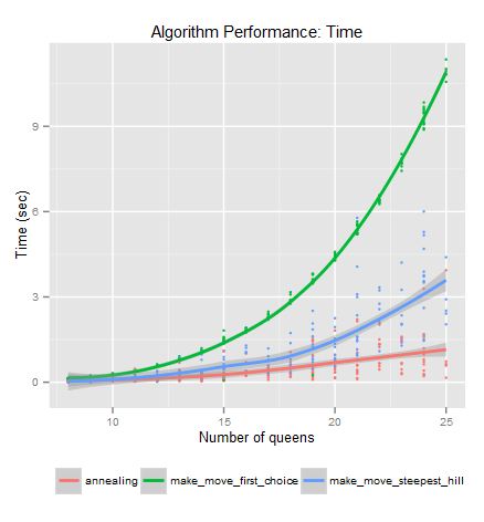
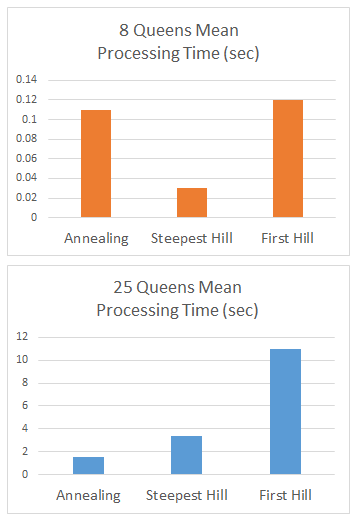
Measuring performance time is the most interesting because the results scale in an obvious pattern. For 8 queens, the clear winner is the steepest hill algorithm. But if we increase the number of queen, both hill climbing algorithms get much slower, while annealing only gets moderately slower:Bar graph of n-queens processing timeBy creating random n-queens puzzles, we can get a very clear picture of how processing time varies with processing time. Consider the following scatterplot:Scatter plot of processing time for n-queensClearly, the first hill algorithm becomes increasingly impractical as the number of queens increases. Steepest hill has a less dramatic increase in time, while annealing only has a modest increase.

This brief look into some searching algorithms should give you some insight into the many considerations that must be made for actual problem-solving tasks. If you’re interested in learning more, I recommend Russell and Norvig’s Artificial Intelligence: A Modern Approach (Amazon affiliate link). They explore many more related algorithms and delve more into the computer science aspects of algorithms.

N-Queens Part 2: More Algorithms

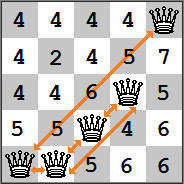
Last time we were considering the following n-queens board with a current heuristic cost of 5:Complete heuristic costs of a given 5-queens puzzle.By making just one move, the best decision would be to move the second queen to the space marked 2. However, to find that move, we had to go through a somewhat expensive algorithm that checks every possible square. What if instead of trying to find the best move at every step, we simply tried to find a better move?

This method of hill climbing is called first-choice hill climbing. Its implementation is simpler than the steepest-hill method:

def make_move_first_choice(board):
	h_to_beat = get_h_cost(board)
	for col in range(len(board)):	
		for row in range(len(board)):
			if board[col] == row:
				#We don't need to evaluate the current
				#position, we already know the h-value
				continue
			
			board_copy = list(board)
			#Move the queen to the new row
			board_copy[col] = row
			new_h_cost = get_h_cost(board_copy)
			
			#Return the first better (not best!) match you find
			if new_h_cost < h_to_beat:
				board[col] = row
				return board
	
	return board

A final algorithm to consider introduces randomness. Since any n-queens state can be reached from any other n-queens state, it is possible that a solution could arise by simply making random moves. However, a purely random algorithm would take a very long time to stumble upon a solution. The annealing algorithm attempts to tease out the correct solution by making risky moves at first and slowly making more conservative moves.

The algorithm builds on the metaphor of real life annealing, a process used in glass blowing and metallurgy. For example, molten glass is extremely hot, but cools fairly quickly. Generally, room temperature is too cold and the glass will end up cracking. To prevent this, glass is placed into an annealing oven that slowly lowers the temperature, ensuring a more stable cooling process. The algorithm uses a “temperature” and “annealing rate” to “cool” the risk. Here is the basic process:

  1. Make a random move
  2. If the move results in a lower heuristic cost, accept the move. Otherwise, asses the risk and determine if it should be accepted. If the move is too risky, reject it, and repeat steps 1 and 2.
  3. Reduce the temperature by a given annealing rate.
  4. Repeat until a solution is found.

Risk is determined using the following:

Given:

  • ΔE = current heuristic cost – new heuristic cost
  • current temperature T

The probability of acceptance is min(1,eE/T)).

Much research has gone into determine the correct numbers to use for these variables, but we can use some basic principles for a simple problem like n-queens. In general, you want to start with a high enough temperature that aims for about 80% acceptance on the first move, and you want to anneal at a rate of about 95%.

import math
import random

def annealing(board):
	temp = len(board)**2
	anneal_rate = 0.95
	new_h_cost = get_h_cost(board)
	
	while new_h_cost > 0:
		board = make_annealing_move(board,new_h_cost,temp)
		new_h_cost = get_h_cost(board)
		#Make sure temp doesn't get impossibly low
		new_temp = max(temp * anneal_rate,0.01)
		temp = new_temp
		if steps >= 50000:
			break

def make_annealing_move(board,h_to_beat,temp):
	board_copy = list(board)
	found_move = False

	while not found_move:
		board_copy = list(board)
		new_row = random.randint(0,len(board)-1)
		new_col = random.randint(0,len(board)-1)
		board_copy[new_col] = new_row
		new_h_cost = get_h_cost(board_copy)
		if new_h_cost < h_to_beat:
			found_move = True
		else:
			#How bad was the choice?
			delta_e = h_to_beat - new_h_cost
			#Probability can never exceed 1
			accept_probability = min(1,math.exp(delta_e/temp))
			found_move = random.random() <= accept_probability
	
	return board_copy

This algorithm is a little more complex and involves two methods, but follow along with the general steps above and it should start to make sense.

Note that it is possible for both of these algorithms to get “stuck”. This is known as a plateau. Therefore, it is usually a good idea to put a cap on the number of attempts the algorithm can make before giving up. In the annealing algorithm, I allowed a maximum of 50000 iterations.

In the next post we’ll look at how these algorithms actually perform and make some generalizations about when certain algorithms excel.

N-Queens Part 1: Steepest Hill Climbing

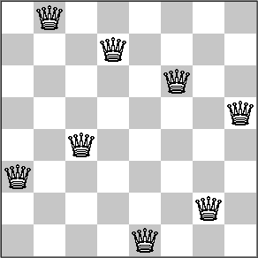
The n-queens problem was first invented in the mid 1800s as a puzzle for people to solve in their spare time, but now serves as a good tool for discussing computer search algorithms. In chess, a queen is the only piece that can attack in any direction. The puzzle is to place a number of queens on a board in such a way that no queen is attacking any other. For example:A diagram of a solved 8-queens problemOne way we can describe this board is to say it has a heuristic cost of 0, because there are 0 pairs of queens attacking each other. We can then generalize this to say the heuristic cost of a given n-queens board is equal to the number of queens directly or indirectly attacking one another. Consider this 5-queens puzzle. There are 5 pairs of queens attacking each other therefore the heuristic cost of this board is 5.An unsolved 5-queens problem. We can calculate the heuristic cost easily if we represent a board as an array where the index is the column and the value is the row. The board above is [0,0,1,2,4].

def get_h_cost(board):
	h = 0
	for i in range(len(board)):
		#Check every column we haven't already checked
		for j in range(i + 1,len(board)):
			#Queens are in the same row
			if board[i] == board[j]:
				h += 1
			#Get the difference between the current column
			#and the check column
			offset = j - i
			#To be a diagonal, the check column value has to be 
			#equal to the current column value +/- the offset
			if board[i] == board[j] - offset 
				or board[i] == board[j] + offset:
				h += 1
		
	return h

To solve this puzzle, we need to take steps to reduce the heuristic cost to zero.

In order to evaluate which moves are best, we can calculate the heuristic cost of the board after one move. This diagram shows the heuristic costs of all possible moves from the current board. For simplicity, we will only move queens up or down in their rows.Complete heuristic costs of a given 5-queens puzzle. If you would choose the move with the lowest heuristic cost and then repeat the process, then you would be using the steepest hill climbing algorithm.

The hill climbing algorithm gets its name from the metaphor of climbing a hill where the peak is h=0. But there is more than one way to climb a hill. If we always choose the path with the best improvement in heuristic cost then we are using the steepest hill variety.

Steepest hill climbing can be implemented in Python as follows:

def make_move_steepest_hill(board):
	moves = {}
	for col in range(len(board)):
		best_move = board[col]
		
		for row in range(len(board)):
			if board[col] == row:
				#We don't need to evaluate the current
				#position, we already know the h-value
				continue
			
			board_copy = list(board)
			#Move the queen to the new row
			board_copy[col] = row
			moves[(col,row)] = get_h_cost(board_copy)
	
	best_moves = []
	h_to_beat = get_h_cost(board)
	for k,v in moves.iteritems():
		if v < h_to_beat:
			h_to_beat = v
			
	for k,v in moves.iteritems():
		if v == h_to_beat:
			best_moves.append(k)
	
	#Pick a random best move
	if len(best_moves) > 0:
		pick = random.randint(0,len(best_moves) - 1)
		col = best_moves[pick][0]
		row = best_moves[pick][1]
		board[col] = row
	
	return board

But as I mentioned above, there are multiple ways to climb a hill! Next time we’ll look at some additional ways to solve n-queens problems.

Finding the colors used in graffiti through clustering

Earlier this week, a Graffiti “museum” of sorts in New York was destroyed. Graffiti artists from around the world came to contribute to the ever-changing murals at 5Pointz.

To combine millions of colors into just 32 obviously removes a lot of variation and vibrancy. But still, this graph gives a strong indication of the overall palette used. For example, notice the inclusion of bright pinks and blues in spite of removing the noise.

I’ve seen average color analyses before and the idea inspired me to investigate the colors present at 5Pointz. The official website has a lot of great photos. I grabbed about a hundred, cropped out sidewalks, sky, etc. and processed them through Python to get the RGB data for each of the pixels. The Python Imaging Library makes this super easy.

import Image

rgb_counts = {}

def get_img_details(image_name):
	image = Image.open("./images/" + image_name)
	width = image.size[0]
	height = image.size[1]
	pixels = image.load()
	for x in range(width):
		for y in range(height):
			rgb = pixels[x,y]
			if rgb_counts.get(rgb):
				rgb_counts[rgb] += 1
			else:
				rgb_counts[rgb] = 1

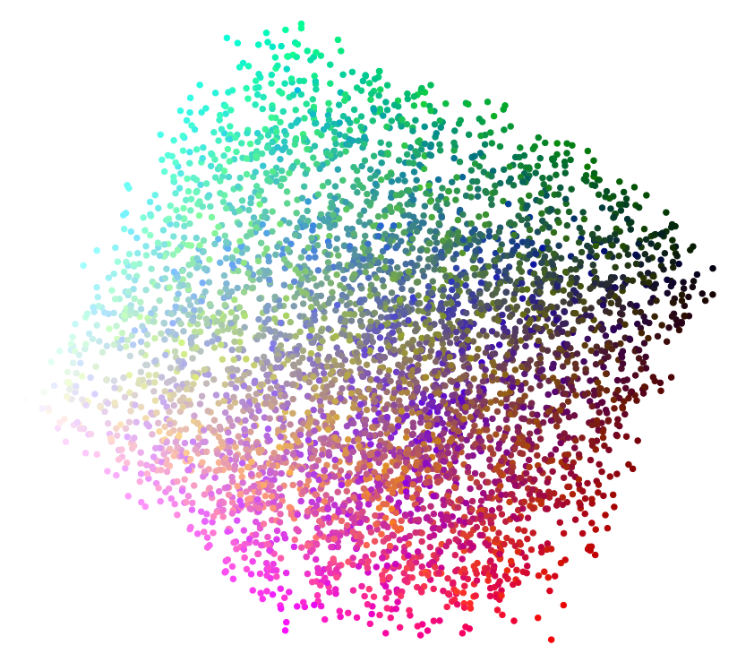
After doing this, there were over 2.5 million unique colors. With so much noise, I wanted to pare down the data to create something visual. For this, I turned to clustering in R to get “average” color pockets. After clustering, the clusterplot function in the fpc library makes this interesting visual of 5000 randomly sampled points.Clusters of colors from graffitiYou can see shades of similar colors grouped together. Finally, I took the red, green, and blue means of each of the clusters to create the graph above.

Full code for this is available here and here.