How quickly can a computer learn Tic Tac Toe?

In my post last week, I discussed my Java implementation of the MENACE Tic Tac Toe machine. I also mentioned how playing against the MENACE manually is simply too time consuming. And since all programmers are lazy, I of course went on to allow two computer players compete against each other.

However, I never really gave MENACE the best chance for success. Playing against a random computer or another MENACE is really just leaving it up to luck. A successful teacher leads to a more successful student. So I also implemented a computer that plays optimally.

There are a few different ways to do this, and a lot of exercises involve using a minimax algorithm with optional alpha-beta pruning. However, that seems like overkill to me. Tic Tac Toe is a “solved” game meaning that we know how to make the best play every time by simply following a set of rules. Implementing these rules was fairly straight-forward.

So now that MENACE had a good teacher, how long did it take to learn the game? Unfortunately MENACE’s lot in life is sad in that it will never win against an optimal teacher. We know this because a perfectly played game is a draw. So for me the way to determine success is by looking at the optimal player’s wins. The fewer number of times the optimal player wins, the faster MENACE is learning. The mechanics as I found them described online are:

  • Win: MENACE gains one bean (+1)
  • Draw: MENACE has no change (0)
  • Lose: MENACE loses one bean (-1)

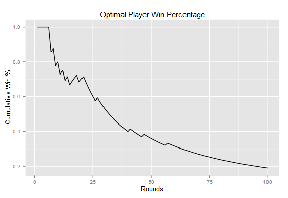
I then ran a simulation of one thousand “tournaments” each consisting of one hundred games. The median number of games the optimal player won was 66. This means on average it took MENACE 66 losses before it could play optimally. This graph shows the cumulative wins the optimal player had in one particular tournament of one-hundred games. The optimal players starts with a 100% winrate, but the winrate slowly drops until the player stops winning all together.

MENACE Cumulative Wins

However, I was not convinced that this training method was best. After all, an optimal player should force a draw which means a draw is actually a positive outcome. However, a win is still yet more positive. I tested my theory with a few different values and found these to be the most effective:

  • Win: MENACE gains two beans (+2)
  • Draw: MENACE gains one bean (+1)
  • Lose: MENACE loses one bean (-1)

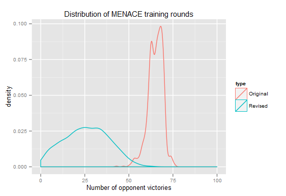
With these values the number of games for optimization was considerably fewer: 26 games. The distribution turned out to be wider mostly because MENACE is more influenced by making lucky or unlucky plays. This graph compares the outcomes of the two tournaments:

Number of wins to train MENACE

This was a fun exploration and there’s still some room for improvement. If you’d like to play with MENACE yourself, the code is available on GitHub.

Java Tic Tac Toe – MENACE

If you’ve ever played Tic Tac Toe, you know that the game gets boring after only a few rounds. The reason for this is because every possible board state has an optimal play. Furthermore, these optimal plays are simple enough to calculate that two optimal players will always cause a draw. The only way to win is if your opponent makes a mistake. Contrast this to a game like Chess where there is rarely a single optimal move. Instead moves must be made off of a series out potential outcomes. Going further, we can consider a game like Go where almost any play can be advantageous depending on the player’s skill. Randall Munroe of xkcd has a nice visual comparison of this concept. (Randall Munroe of xkcd also has nice visual comparison of the optimal tic tac toe plays!)

A few months ago, I came across this great article by James Bridle. In it, he describes a mechanical system (Matchbox Educable Noughts And Crosses Engine) designed by Donald Michie to “play” Tic Tac Toe and learn the rules without any information about how to win.

But what’s really clever is that MENACE learns. Every time it wins a game, an additional bead is added to each matchbox played, corresponding to each winning move. Likewise, every time it loses, a bead corresponding to each losing move is removed. As a result, over time, MENACE becomes more likely to play moves that have previously resulted in wins and less likely to play moves that have resulted in losses.

The concept is simple enough that I decided to make a computer implementation of MENACE.

The Code

Unlike a traditional Tic Tac Toe “AI”, the purpose of this implementation is that the computer player does not know the rules of the game. The only “rules” it knows about are:

  • Certain moves are illegal (but no explanation is given as to why they are illegal)
  • The game ends
  • The outcome is either win, lose, or draw

When it is the computer’s turn to play, it checks to see if it has a record of the current board state. If it does, it plays the move that has the highest score (number of beans). Otherwise, it plays randomly.

    private int retrieveOptimalPlayLocation(BoardState bs)
    {
        //Find matching board state
        BoardState matchingState = retrieveKnownBoardState(bs);
        //Find the highest value in the array
        int[] bsCounter = null;
        
        if(rank == playerRank.ALPHA)
        {
            bsCounter = Arrays.copyOf(matchingState.getPlayerAlphaLogicCounter(),9);
        }
        else if(rank == playerRank.BETA)
        {
            bsCounter = Arrays.copyOf(matchingState.getPlayerBetaLogicCounter(),9);
        }
        Arrays.sort(bsCounter);
        int optimalPlayValue = bsCounter[8];
        
        //Find a play with the highest value
        if(rank == playerRank.ALPHA)
        {
            bsCounter = matchingState.getPlayerAlphaLogicCounter();
        }
        else if(rank == playerRank.BETA)
        {
            bsCounter = matchingState.getPlayerBetaLogicCounter();
        }

        int optimalPlayLocation = -1;
        boolean bestPlayFound = false;
        
        //It's possible that multiple plays are equal. 
        //This picks a random best play.
        while(!bestPlayFound)
        {
            int randomEntry = r.nextInt(9);
            int playValueToCheck = bsCounter[randomEntry]; //Select a random play
            if(playValueToCheck == optimalPlayValue && checkPlayAvailable(bs, randomEntry))
            {
                optimalPlayLocation = randomEntry;
                bestPlayFound = true;
            }
                
        }
        return optimalPlayLocation;
    } 

After each round, the computer updates its “matchboxes” based off of the outcome of the round.

    public void processEndOfRound()
    {
        Player lastToPlay;
        if(turns % 2==0)
            lastToPlay = player2;
        else
            lastToPlay = player1;

        BoardState boardToUpdate;
        int logicAmountChange = 0;

        if(victory && lastToPlay instanceof HumanPlayer) //Human wins
        {
            System.out.println("You won in " + turns + " moves!");
            logicAmountChange = -1;
            
        }
        else if(victory && lastToPlay instanceof ComputerPlayer) //Computer wins
        {
            System.out.println("The computer won in " + turns + " moves!");
            logicAmountChange = 2;
        }
        else //Draw
        {
            System.out.println("The game ended in a draw.");
            logicAmountChange = 1;
        }
                
        for(int[] turn : moveHistory)
        {
            if(turn[0]!=0)
            {
                boardToUpdate = BoardStateChecker.getKnownBoardStates().get(turn[0]);
                boardToUpdate.changeLikelihood(turn[1],
                        logicAmountChange, 
                        ((Game_HvC)theGame).getComputerPlayer().rank);
            }
        }

    }

You can view the full source code over at GitHub.

When I first put this together, I wanted to test it with me playing against the computer. It worked, but only if I played reliably. Any deviation results in a new board pattern that the computer doesn’t know about. To really see a computer player “learn”, I implemented two additional game modes: learning computer vs. random computer and learning computer vs. learning computer. This allows the two players to play a few thousand games in just about a second and get stats about the game outcomes. In my next post, I’ll share my findings and stats from these automated game play modes.

Coursera Data Analysis Review

I recently completed the Coursera course Data Analysis (Winter 2013) presented by Professor Jeff Leek. For those of you unfamiliar with the format, a MOOC (massive open online course) is a university-level course taught online to anyone who signs up and participates. Usually the lectures are in video format and there and quizzes and sometimes projects to score students’ performance.

A ton of work goes into putting together a MOOC and I have a lot of respect for all the staff involved. Additionally, these courses are 100% free. This makes it a bit problematic to criticize because I have invested nothing other than my time which I did so willingly. Nonetheless, the universities and companies who create these courses do so for a reason and I believe they are always looking to improve and better themselves. I felt that most salient problems in the class can be boiled down to two “challenges” with the MOOC format. These are not revolutionary criticisms, but I hope they add to the discussion on this new format of learning.

The phrase “Data Analysis” can mean hundreds of different things so I found it surprising that the class did not have a subtitle or specific focus. Yet in eight weeks, we covered a lot of material and were exposed to lots of high-end analysis techniques. In reading feedback on the class forums, the pacing of the course seemed to be contentious for many students. This brings me to the first challenge: a diverse student body. Diversity is almost always good as it fosters ideas and discussion. However, most university courses have prerequisites to make sure everyone in the class is on an even playing field. In a MOOC anyone with an Internet connection can participate. While I’m all for continued openness, I felt this class could have benefited by being more clear upfront about necessary knowledge. It seems as if many students were trying to learn R and/or basic statistics while taking this class. To me this seems like jumping into calculus hoping to pick up algebra on the way. I know Cousera wants to encourage participation, but they shouldn’t be afraid to be honest about course requirements.

The reason I don’t think MOOCs will ever replace college is the barrier between the professor and the students. Getting direct feedback on a paper or an answer to your specific question is the real value of in-person classes. That’s simply not possible in a MOOC. For this class, feedback was available from three places: quizzes, analysis papers, and the forums.

The quizzes are graded automatically and instantly upon submission and are great for quickly assessing your understanding of the lecture material. I like this format and I really think it works well. One suggestion is to have a “hint” button that offers a nudge in the right direction or a link back to the relevant lecture slides.

The data analysis projects gave us a chance to work with real data and apply techniques learned I the lectures to the data. This is a great idea, but in practice cannot succeed. The feedback on these projects came from other students in the class. While a peer grader can evaluate a statement like “Did the paper have sections X, Y, and Z?” how can I trust a peer grader to evaluate questions like “Were the correct statistical methods applied?” or “Did the author draw correct conclusions based on the analysis?” Even I felt a bit uneasy while grading my peers’ papers. Maybe I think the student did something wrong when really it was me who was wrong. Maybe we’re both wrong but I score the paper well because I did the same thing. I believe every paper gets scored by thee or four peers which should help to normalize errors, but that’s no guarantee of accuracy.

Finally the forums were the last place to get feedback. I found them useful when a quiz was worded poorly or even for reading through some ideas that other students were considering for their papers. Unfortunately, there is not really any way to trust the accuracy of the information. The professor occasionally commented, but usually more on course technicalities instead of content questions. There were a few community TAs, but they were fellow students and it seemed like they didn’t really have much access to the professor. It would have been better if a few grad students actually working for the professor were TAs and were able to give authoritative answers to questions. Honestly much of the communication between the TAs and students was arguing.

These three methods highlight the second challenge: feedback. Learning is difficult without feedback and I feel this course’s biggest downside was the lack of available feedback. I think a much better format would be like what I have seen in a few Udacity classes. The student enters information or code, or answers a question that is then instantly graded before moving on. Sometimes they are quick knowledge checks and other times they are longer application exercises. In either case, after answering (right or wrong) you get an immediate explanation detailing the correct answer/approach. This is much more constructive than getting a grade back from a peer who may or may not understand the material himself.

Professor Leek offered his thoughts about the class on the Simply Statistics Podcast and I was happy to see they brought up many of the same issues discussed here. I don’t think I agree with the necessity of a data analysis project in its current format. Certainly writing about and presenting conclusions is important, but the methods of doing so will be different for every different person depending on their field. If I gave a manager in the private sector a report in the style of an academic analysis, his eyes would glaze over. Especially in a course this short, I think communication skills should be left out in favor of focusing on the core content.

In the end, however, what is most important is if I learned something and I can definitely say I did learn from this course and I was exposed to several new and interesting techniques for analysis. I hope to see this course offered again with some improvements. Hopefully many of the students who were too discouraged to complete the course the first time around will consider revisiting it a second time. There is a lot of potential to MOOCs and I look forward to taking more in the future.

How to get to the Project Runway finale

I recently saw this hazard rate analysis of RuPaul’s Drag Race and was inspired to do some analysis on the one reality show I watch:  Project Runway.

I’ve found that the downsides to hazard rates is that they are very inaccurate when you have small data sets and also on the “edge” of the time series. Instead of a hazard analysis, I decided to look at the factors that determine success on Project Runway.

I gathered biographical data from the BravoTV and MyLifetime websites and show outcome data from Wikipedia. There have been 155 regular season contestants and I used 113 in my training data set and 42 in my testing data set. There’s not enough data to predict past winners (there have only been 10 seasons), but there was enough for me to predict past finalists.

For each finalist, I gathered their age; sex; city of residence population; education; if the designer has their own line; raw number of wins, high scores, safe scores, and low scores; and percent of wins, high scores, safe scores, and low scores. (Data available here.)

Using the tree library for R, I fit a tree with the following model:

library(tree)
pr<-read.table("clipboard",sep="\t",header=T)
pr$popcut<-cut(log(pr$Population),6)

##Generate random samples to split dataset
tf<-as.logical(rbinom(155,1,.8))
prtrain<-pr[tf,]
prtest<-pr[!tf,]

##Make the tree model
prt<-tree(PlacedSeason ~ Age + popcut + Win + High + 
    Safe + Low + WinPct + HighPct + SafePct + LowPct

##Prune to compensate for over-fitting:
prt.prune<-prune.tree(prt,4)

Surprisingly, the model ended up needing just two variables: number of wins and number of high scores. Here’s the visual version of the tree. Decision trees are read by evaluating the statement and if it is true going to the left and if it is false going to the right.

Project Runway Decision Tree

Decision tree for Project Runway finalists.

This model was 88% accurate on the test data set. Here’s where it made mistakes:

NameSeasonResultPredictedWinHighSafeLow
Austin Scarlett1Went HomeFinalist2015
Jerell Scott5Went HomeFinalist3342
Carol Hannah Whitfield6FinalistWent Home1470
Mila Hermanovski7FinalistWent Home1336
Sonjia Williams10Went HomeFinalist3242
Fabio Costa10FinalistWent Home1453

The question that you might be asking is can we predict successful designers before the season starts? I looked at the age, sex, city of residence population, education, and if the designer has their own line, but unfortunately did not find a successfully predictive model. That would suggest that the show is mostly about design skill and personality and not about the designers’ backgrounds.

That being said, does the model suggest anyone go to finale now that season 11 has started? As it turns out, the model would predict Daniel to go to the finale because of his two wins. Richard and Stanley are the next closest based on their one win and three high scores (each). However, its also possible the team dynamic of this season makes the model invalid. I couldn’t find any Vegas odds for Project Runway, by money is on Daniel, Stanley, and Michelle.

Bach and Mozart by the Notes

I am a big fan of classical music and while listening to Bach the other day, I wondered if it would be possible to get numerical data on the actual notes used by a particular composer.

I remember as a kid I used to download MIDI files and was always fascinated how programs could read MIDIs into visual notes. MIDI data is encoded into byte chunks where each chunk includes a “command” like “start playing note” followed by the data chunk. In my case, I wanted to read just the data related to the actual notes. This was easy enough to do using the Java MIDI library. This is the workhorse class I put together to get out the note information:

Reading note information from MIDI in Java

package midireader;

import java.util.ArrayList;
import java.util.List;
import javax.sound.midi.ShortMessage;

public class MIDIAnalyzer
{
  private static final String[] sharpNoteNames =
    {"C", "C#", "D", "D#", "E", "F",
        "F#", "G", "G#", "A", "A#", "B"};
  private static final String[] flatNoteNames =
    {"C", "Db", "D", "Eb", "E", "F",
        "Gb", "G", "Ab", "A", "Bb" ,"B"};

  //Each track of the MIDI has
  //its own array of ShortMessages
  private ArrayList<ShortMessage[]> messages;

  public MIDIAnalyzer(List<ShortMessage[]> messages){
    this.messages = (ArrayList) messages;
  }

  private int[] countNotes(ShortMessage[] smArray){
    int[] notes = new int[12];

    for(ShortMessage sm : smArray){
      if(sm != null){
        if(sm.getCommand() == ShortMessage.NOTE_ON){
          //Taking mod 12 removes the octave information
          notes[sm.getData1() % 12]++;
        }
      }
    }

    return notes;
  }

  public void noteCountSummary(){
    int[] notes = new int[12];

    for(ShortMessage[] smArray : messages){
      int[] trackNotes = countNotes(smArray);
      for(int i = 0; i < trackNotes.length; i++){
        notes[i] = notes[i]+trackNotes[i];
      }
    }

    for(int i = 0; i < notes.length; i++){
       System.out.println(sharpNoteNames[i] +
          "\t" + notes[i]);
		}
  }
}

With this code written, it was time to go back to my roots and download a bunch of MIDIs.

Notes Analysis

I wanted to compare two composers from different eras to see if there were any detectable stylistic differences based on the note selection. I chose Bach and Mozart who were both prolific (i.e. lots of data) and quintessential examples for their respective eras.

To control for key difference, I only downloaded pieces labelled as G Major. My dataset had 128,280 notes written by Bach and 131,107 notes written by Mozart.

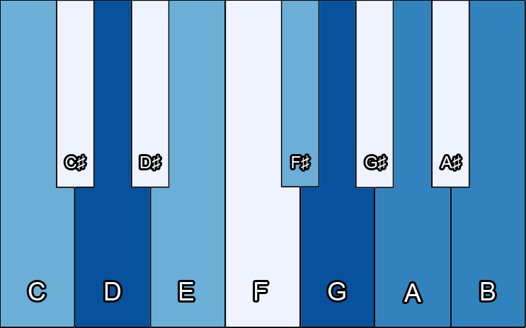
Here is a display of the two composers’ note usage (click to enlarge):

Bach's note usage from G-Major works.

Bach’s note usage from G-Major works.

Bach's note usage from G-Major works.

Mozarts’s note usage from G-Major works.

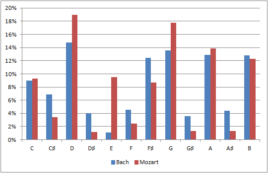
And this compares each composers’ note percentages:

Note comparison graph

Comparison of Bach and Mozart’s note selections.

If you’re unfamiliar with music, in a G-major piece, we would expect to hear lots of G,A,B,D, and F#. This is because the combinations G-D-B and D-F#-A sound good together. Notice that the D is the similar note between each chord and it kind of ties them together. This is why both composers use D the most. You can see that the other four notes are high in both distributions.

What I find most interesting is that Bach’s notes tends to be more spread out. Bach’s pieces often modulate through different keys even from one measure to the next so we see more instances of D♯ and G♯, for example. Mozart on the other hand sticks more closely to the notes of the title key (G major). However, Mozart makes a lot more use of E which can be a major sixth or a relative minor first depending on how it is used. It’s really surprising to me how infrequently this note shows up for Bach. Maybe someone who know more about music than I can let me know why this is.

I would like to look into some later composers and see how the different notes are distributed. I would expect the note counts to be more even as atonality and twelve-tone music became more popular in the 20th century.